Determinantal Point Processes: a quick introduction
November 25, 2018
What’s a point process?
A point process is a random subset of a ground set. For example, if your ground set is \(\left\{ apple, banana, orange, mandarine \right\}\), then a realisation might be \(\left\{ apple, banana \right\}\), another might be \(\left\{ mandarine \right\}\), etc.
A point process might exhibit “attraction”, or it might exhibit “repulsion”. Let’s say \(mandarine\) and \(apple\) are quite different, but \(mandarine\) and \(orange\) are pretty similar. A point process has attraction if mandarine and orange tend to appear together in the subset, and it has repulsion if the opposite is true (if orange is selected, then mandarine likely isn’t). A process that has neither attraction nor repulsion is independent, and we call it a “Poisson point process”.
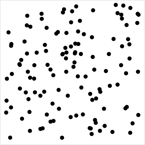
A (discrete) subset of the square is just a bunch of locations on the square. A sample from a Poisson point process looks like this:
A sample from a point process with attraction might look like this:

And a sample from a point process with repulsion might look like:

You may notice how the repulsive point process covers the square much more evenly than the independent (Poisson) point process, which in turn does much better than the attractive point process.
Why repulsion is good (sometimes)
A common way of dealing with the problem of having too much data is to throw some of it away. More optimistically put, one can focus on a random subset of the data, one that is (hopefully) representative of the whole. In the set of fruits we mentioned earlier, if you had to pick a representative sample of size three, it probably wouldn’t contain both \(orange\) and \(mandarine\): in such cases what we need is a repulsive point process.
DPPs are a kind of point process with repulsion. They come from statistical physics (the earliest reference I know of is Macchi, 1975) but they have been popularised in Machine Learning by Kulesza & Taskar.
What’s a DPP?
Let’s say we have \(n\) objects, labelled \(1\) to \(n\). Our goal is to find a sub-sample of size \(k\), much smaller than \(n\). That sub-sample should be picked such as to exhibit high diversity, meaning we don’t want to include items that are too similar.
That calls for a mathematical definition of similarity: we give each pair of items a similarity score \(L_{ij}\) between 0 and 1. \(L_{ii}=1\), so that an item is maximally similar to itself. If two items are completely dissimilar than \(L_{ij}=0\). We can stick all scores into a large \(n \times n\) matrix \(\mathbf{L}\) with entries \(L_{ij}\). An important, but technical, requirement is that \(\mathbf{L}\) should be positive definite (and all its principal minors too).
Now let’s consider a subset of items, noted \(\mathcal{X}\), of size \(k\). We can form a smaller matrix, \(\mathbf{L}_{\mathcal{X}}\) of size \(k \times k\).
We are now almost ready to define DPPs: as noted above, a point process is just a probability distribution over subsets. The next step is simply to define the probability of picking subset \(\mathcal{X}\): in DPPs this is just
\[p(\mathcal{X}) \propto \det \mathbf{L}_\mathcal{X}\]
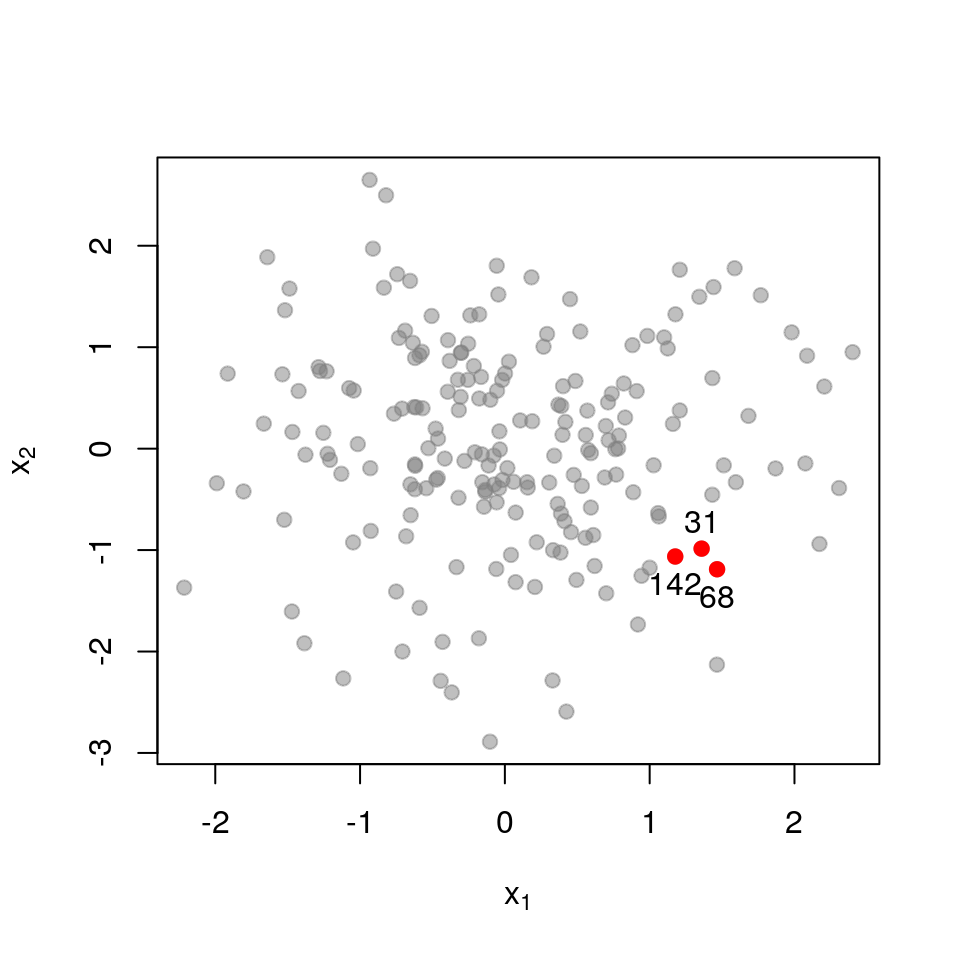
The next few images should help understand why this defines a repulsive point process. We start with \(n=200\) points in the plane.
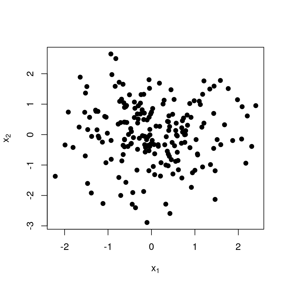 To define the similarities, we pick the traditional Gaussian kernel:
\[ L_{ij} = \exp \left( - \frac{1}{2l^{2}} || \mathbf{x}_{i}-\mathbf{x}_{j} ||^{2} \right) \]
so that points close together are judged to be similar, and points far apart dissimilar.
For purposes of illustration, let’s say we wish to retain only \(k=3\) points out of the original set.
Here is the sub-matrix \(\mathbf{L}_{\mathcal{X}}\) for three points that quite far apart:
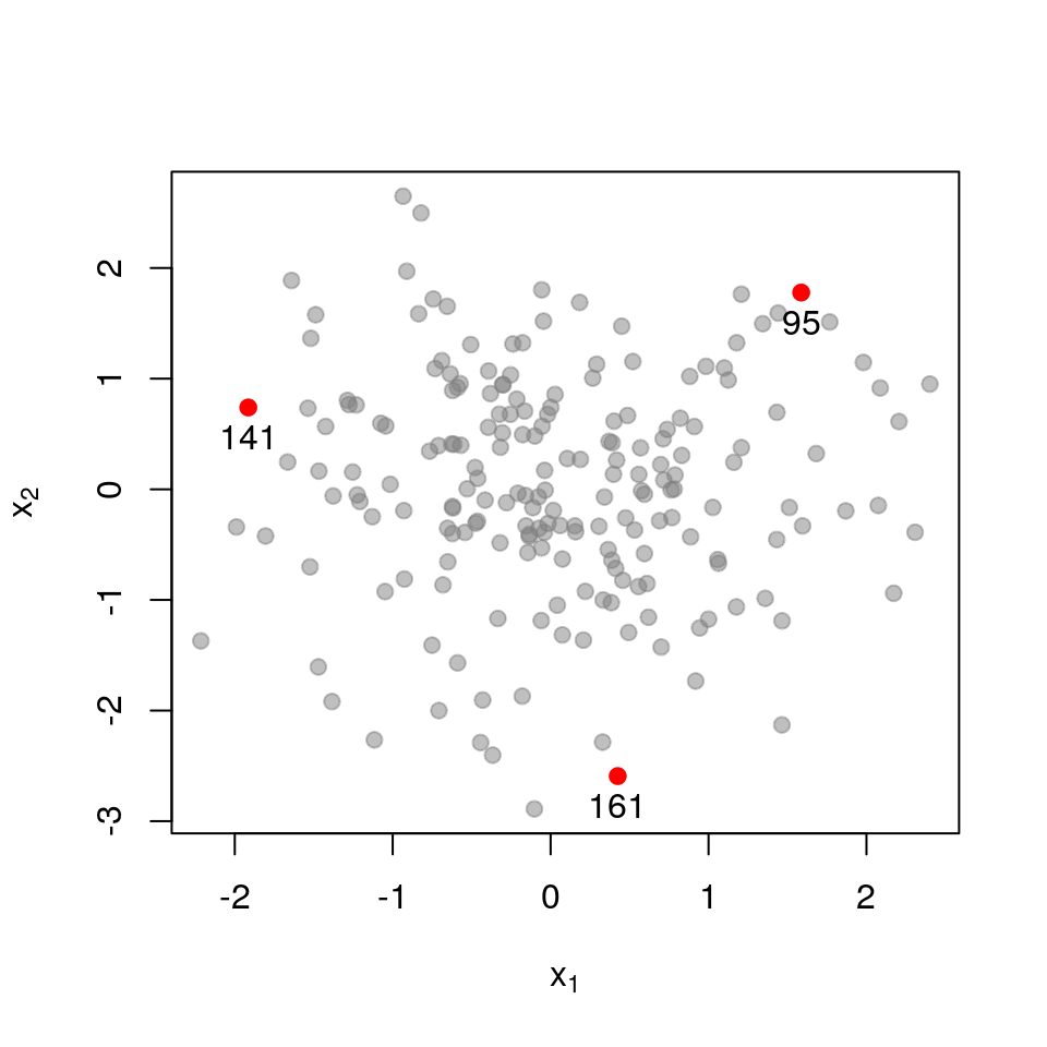
\[ \mathbf{L}_{\mathcal{X}}= \begin{pmatrix} 1.000 & 0.000 & 0.000 \\ 0.000 & 1.000 & 0.000 \\ 0.000 & 0.000 & 1.000 \\ \end{pmatrix} \] \[ \det \mathbf{L}_{\mathcal{X}}= 1.000 \]
The matrix almost equals the identity matrix, and thus has determinant very close to \(1\), the maximum possible value.
Next, a set of points that are closer together:
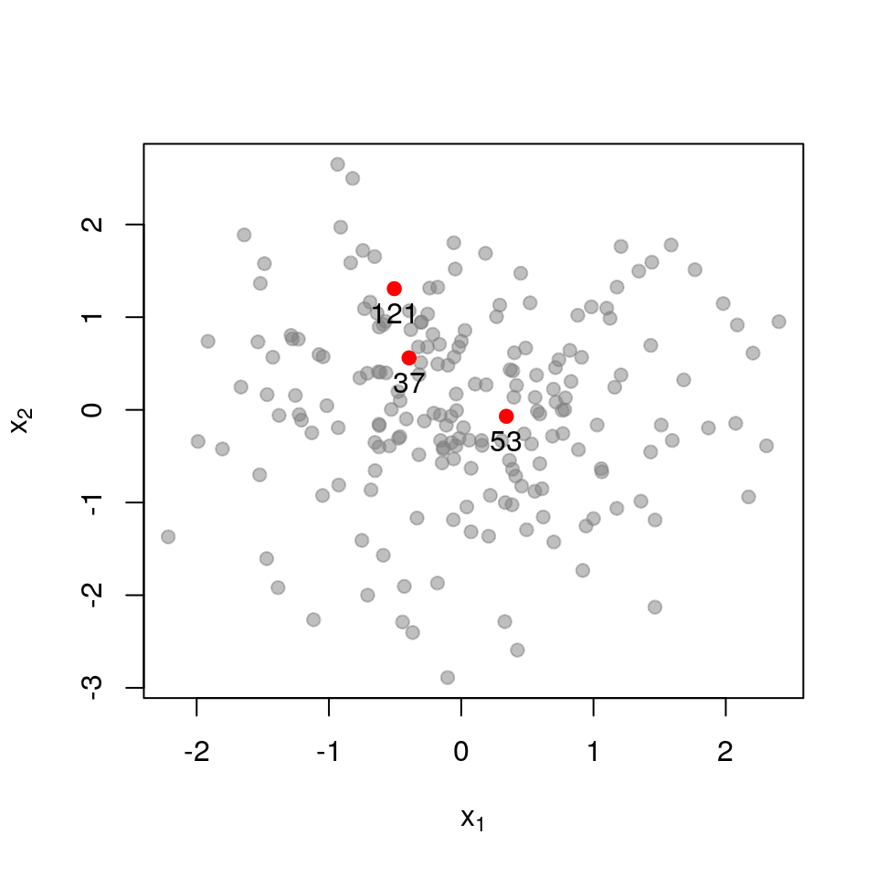
\[ \mathbf{L}_{\mathcal{X}}= \begin{pmatrix} 1.000 & 0.391 & 0.565 \\ 0.391 & 1.000 & 0.073 \\ 0.565 & 0.073 & 1.000 \\ \end{pmatrix} \] \[ \det \mathbf{L}_{\mathcal{X}}= 0.554 \]
Recall that the determinant measures the volume spanned by the column vectors of the matrix (here, vectors in \(\mathcal{R}^{3}\)). The more co-linear the columns are, the lower the determinant. If we now examine a set of points that are very close together, each column in \(\mathbf{L}_{\mathcal{X}}\) almost equals that all-ones vector.
The determinant is below 0.01, meaning that this set of close-together points is 100 times less likely to be picked that a set of far-apart points (for which the determinant is close to 1).
That’s essentially all we need to define a DPP: to verify that \(p(\mathcal{X}) \propto \det \mathbf{L}_\mathcal{X}\) defines a valid probability, we just need to check that all determinants are positive, which is the technical requirement we stated above.
Realisations from the DPP
Here are a few realisations of the DPP we’ve just defined, this time with \(k=20\)
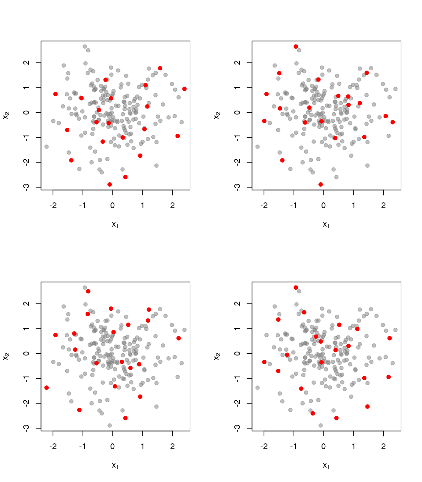
As a comparison, here is what things look like when we just pick uniformly among sets of size \(k=20\):
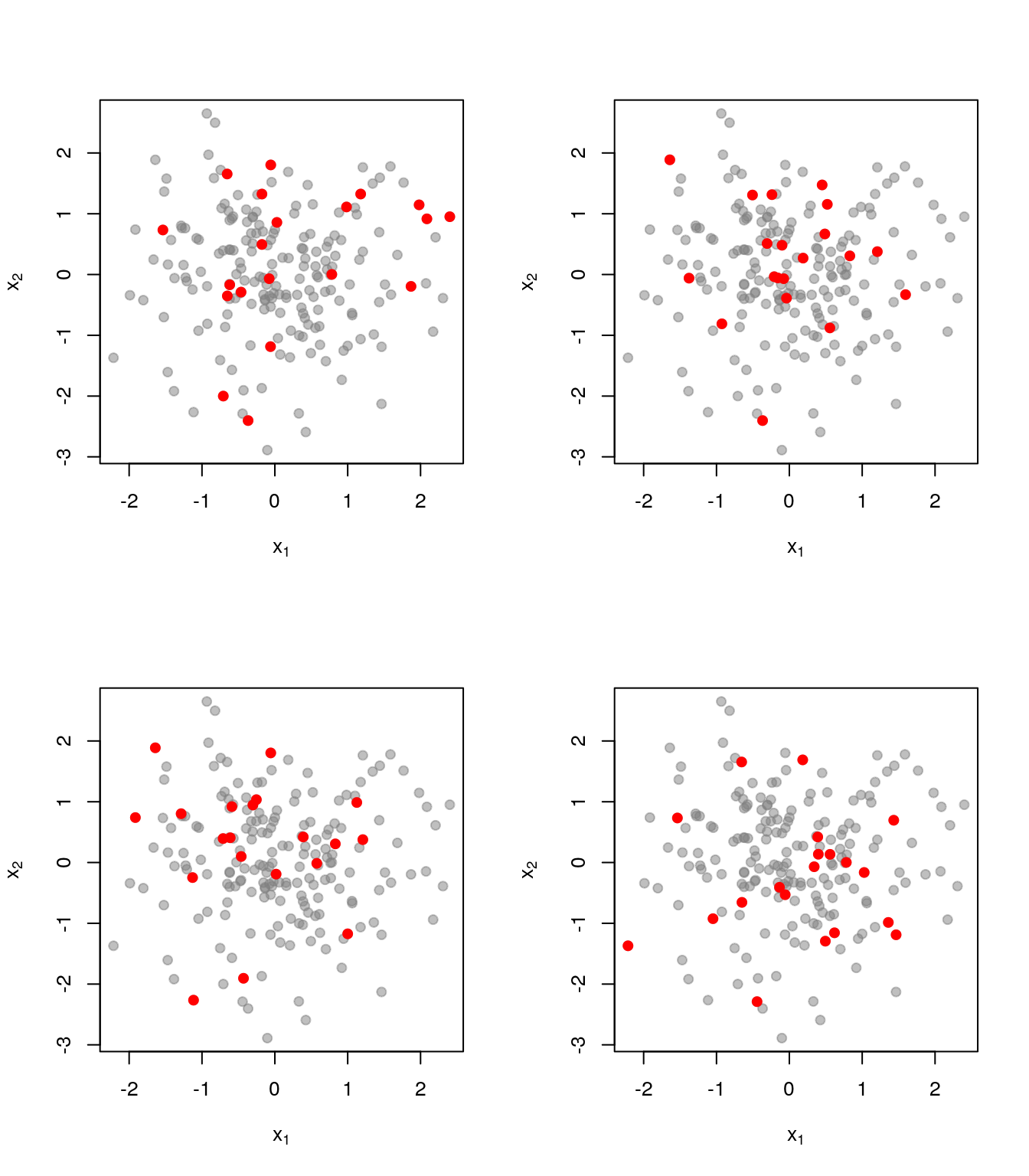
Realisations from a DPP cover the ground set much better.
How to sample from a DPP?
Sampling from a DPP is easy but the algorithm takes a bit of work to derive, see: - Tremblay, N., Barthelme, S., & Amblard, P. O. (2018). Optimized Algorithms to Sample Determinantal Point Processes. arXiv:1802.08471.
For sampling algorithms in Python see DPPy.
Here’s a dead-simple, but unoptimised, MCMC sampler in R:
library(purrr)

#Sample a k-DPP using MCMC
#This is an MCMC algorithm, not an exact sampler. Remove the early samples (burn-in), after that you should have a DPP
#Input: the L-matrix (size nxn). k: size of DPP subset. nSamples: number of MCMC samples
dpp.mcmc <- function(L,k,nSamples=10*k)
{
    n <- nrow(L)
    S <- matrix(NA,nSamples,k)
    #Initial set
    set <- sample(n,k)
    ldet <- logdet(L[set,set])
    for (indS in 1:nSamples)
    {
        #Pick an index to update
        ii <- sample(k,1)
        #Remove item ii, insert new item
        newitem <- sample(setdiff(1:n,set[-ii]),1)
        nset <- c(set[-ii],newitem)
        ldet.new <- logdet(L[nset,nset])
        if (log(runif(1)) < ldet.new - ldet) #Accept new set
        {
            set <- nset
            ldet <- ldet.new
        }
        S[indS,] <- set
    }
    S
}

#Stable evaluation of log-determinant
logdet <- function(K)
  {
    2*sum(log(diag(chol(K))))
  }

#Example: ground set
X <- matrix(rnorm(500*2),500,2)
#L-matrix
L <- dist(X)  %>% as.matrix  %>% { exp(-.^2) }

S <- dpp.mcmc(L,20,nSamples=500)[-(1:400),]
#Plot ground set
plot(X,pch=19)
#Highlight DPP samples
points(X[S[1,],],col="red",pch=19)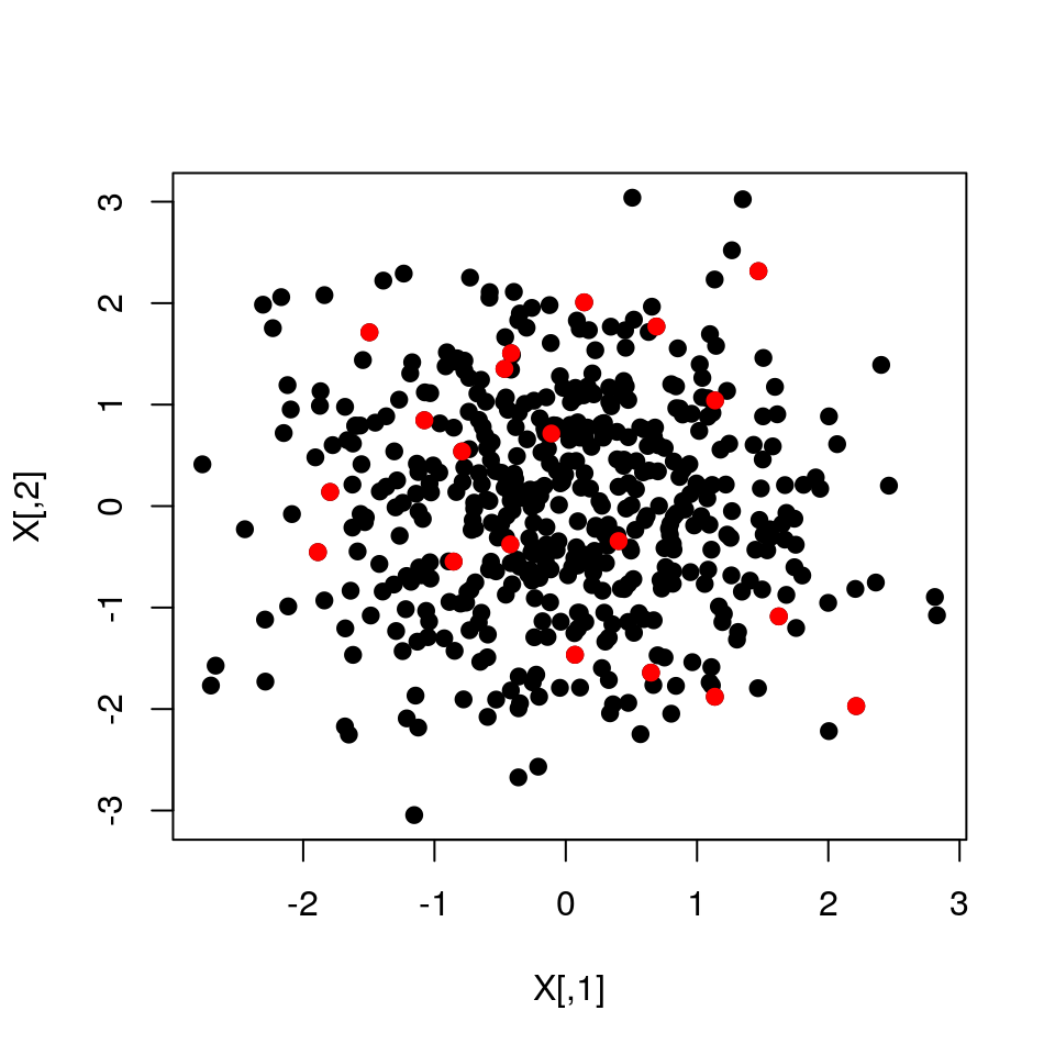
The beauty of DPPs
DPPs are not the only repulsive point processes around. What’s nice about DPPs is that they are tractable: you can easily sample realisations, but you can also compute inclusion probabilities. An inclusion probability is the probability of finding item \(i\) in the random subset: importance sampling requires inclusion probabilities. For much more than you wanted to know on inclusion probabilities in DPPs, see:
- Barthelmé, S., Amblard, P. O., & Tremblay, N. (2018). Asymptotic Equivalence of Fixed-size and Varying-size Determinantal Point Processes. arXiv:1803.01576
Another fascinating aspect of DPPs, from a theoretical stand-point, is that they crop up all over the place: in statistical physics, in random matrix theory, in graph theory, and probably other places. Kulesza & Taskar have a list of things that turn out to be DPPs.
Applications
There are many, as a quick search will reveal. We ourselves have worked on applying DPPs to graphs (for sampling nodes), see:
- Tremblay, N., Amblard, P. O., & Barthelmé, S. (2017) Graph sampling with determinantal processes. In Signal Processing Conference (EUSIPCO), 2017 25th European (pp. 1674-1678). IEEE. arXiv:1703.01594
Another interesting application is to use DPPs to form coresets, which are subsets that are provably good for learning:
- Tremblay, N., Barthelmé, S., & Amblard, P. O. (2018). Determinantal Point Processes for Coresets. arXiv:1803.08700.